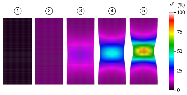
Curve and Image Sequence

Image sequence synchronized with a response curve.

import clearplot.plot_functions as pf
import matplotlib.pyplot
import os
import numpy as np

#Load global response
data_dir = os.path.join(os.path.dirname(pf.__file__), os.pardir, 'doc', \
    'source', 'data')
path = os.path.join(data_dir, 's140302C-mechanical_response.csv')
data = np.loadtxt(path, delimiter = ',')
#Specify the indices of the field images to be plotted
ndx_list = [0, 85, 141, 196, 252]
#Specify the column indices to crop the images to
cols = range(470,470+340)
#Load the field images into an image sequence list
im_seq = []
for ndx in ndx_list:
    #Load field image
    im_filename = 's140302C-eqps_field-frame_%r.png' %(ndx)
    im_path = os.path.join(data_dir, 'hi-rez_field_images', im_filename)
    im = matplotlib.pyplot.imread(im_path)
    #Crop the field image and add to list
    im_seq.append(im[:,cols,:])
#Create labels
labels = []
for i in range(1, len(ndx_list) + 1):
    labels.append(str(i))

#Plot curve
[fig, ax, curves] = pf.plot('', data[:,0], data[:,1], \
	x_label = ['\varepsilon', '\%'], y_label = ['\sigma', 'GPa'])
ax.label_curve(curves[0], labels, ndx = ndx_list, angles = 60)
ax.plot_markers(data[ndx_list,0], data[ndx_list,1], colors = [0,0,0])
fig.save('curve_and_image_sequence-a.png');
#Plot image sequence
[fig, ax, im_obj] = pf.show_im('curve_and_image_sequence-b.png', \
    im_seq, scale_im = 0.3,  c_label = ['\bar{\varepsilon}^p', '\%'], \
    c_lim = [0, 100], c_tick = 25, b_labels = True, im_interp = 'bicubic', \
    c_bar = True);

Curve:

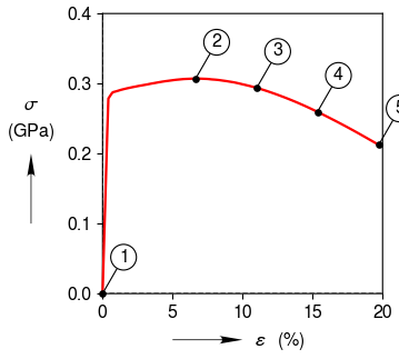
Image Sequence: